Home

Diffraction Pattern of Obstructed Optical Systems

With the only exception of the "Schiefspiegler" (Oblique Telescope, like the design by Anton Kutter) every Telescope with the main objective being a mirror is obstructed, and the quality of the image suffers more or less from the resulting disturbance of the diffraction pattern. As a rule of thumb we have learned, that a central obstruction of less than 20% (linear diameter) is negligible for the quality of the resulting image.
But what is the effect of more complicated obstructions, like thick vanes carrying the secondary mirror or other constructive elements that protrude into the optical path? Since this may be an important question when planning and constructing telescopes and other optical instruments, I ran some simulations to get an idea of the influences on image quality.

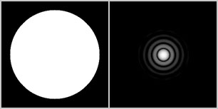
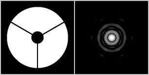
Figure 1shows the simulated diffraction pattern (= Airy disk, right) that would result from a circular unobstructed opening (left) in monochromatic light. The diffraction pattern is diplayed in a logarithmic gray scale as it would be seen by the human eye with a scaling from black to white of eight astronomical magnitudes (8 mag.) The field of the simulated views is 6" (arcseconds) wide.This will be true for all the following simulated diffraction pattern unless other stated.

Figure 1a: Diffraction Pattern (Airy disk, right) of an unobstructed circular entrance pupil (left), like from a Refractor or a Schiefspiegler. The field of view is 6" (arcseconds) wide.

If we know the energy distribution in the diffraction pattern, we are able to simulate the image that would result from imaging an object with an instrument with exactly this entrance pupil but an otherwise perfect optical system. 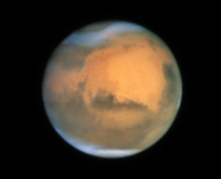This gives us the opportunity to compare the influence of obstructions on the image quality bare from different optical conditions of the instruments used normally for such side by side tests. I used Mars (an image from the Hubble Space telescope) as test-object, since its surface with the many low contrast features of different size is very sensible to a decrease in image contrast of the optical instrument.

Figure 1b: Simulated view of Mars with the unobstructed optical system from Fig.1a at a diameter of the entrance pupil (=objective diameter) of 400mm. The apparent diameter of Mars was assumed to be 20" (arcseconds).

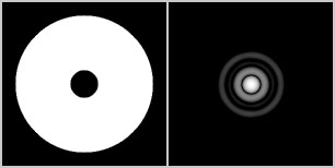
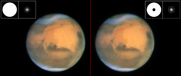
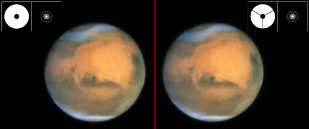
As already mentioned, we have learned that a central obstruction of 20% (Fig. 2a) is negligible for the image quality in most cases. The simulated view in Figure 2b tells the same: the left image is for an unobstructed instrument, the right one is with 20% central obstruction. Virtually no loss in conrast is noticeable.

Figure 2a: 20% central obstruction (left) and the resulting diffraction pattern.

Figure 2b: Mars, imaged with an unobstructed Instrument (left) and an Instrument with 20% central obstruction (right). The resulting image contrast and visibility of surface structures is nearly identical. At the top, the entrance pupil and the resulting diffraction pattern is shown. The pattern is displayed at actual size with respect to the images of Mars.

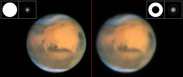
This clearly changes, if we introduce 33% (Figures 3a and 3b) or 50% (Figures 4a and 4b) central obstruction. More light falls into the outer diffraction rings, lowering the contrast of the image. Sometimes you hear the statement, that an instrument with 30% central obstruction is unusable for high magnifications and planetary observations.This is simply not true, as can be seen in the simulated views, and if a central obstruction of about 30% is needed for constructive reqirements, I would not hesitate to build the instrument this way.

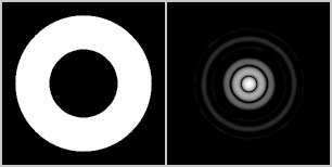
Figure 3a: 33% central obstruction (left) and the resulting theoretical diffraction pattern.

Figure 3b: Mars, imaged with an unobstructed Instrument (left) and an Instrument with 33% central obstruction (right).

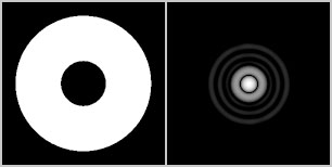
At 50% central obstruction (Fig 4a and Fig. 4b) the loss in contrast is distinct. On the other hand, one can imagine that even this difference should be difficult to figure out at a side by side test, if the conditions of the instruments under test (state of collimation, temperature aclimatisation) are not identical.

Figure 4a: 50% central obstruction and the resulting diffraction pattern

Figure 4b: An instrument with 50% central obstruction (right) again compared to the image with an unobstructed instrument (left). The difference in surface contrast is clearly visible.

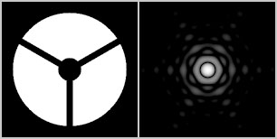
More interesting than the central obstruction, that has been discussed rather often, is the influence of the vanes that carry the secondary mirror. In the Figures 5a and 5b the influence of vanes of 6mm thickness on a 400mm instrument (that is 1.5%) is simulated. Normally vanes are thinner than that.

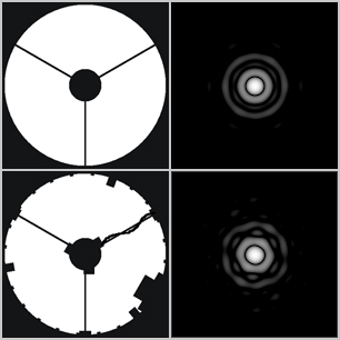
Figure 5a: A three vane spider that is 1.5% of the diameter of the main mirror thick, combined with a central obstruction of 20%.

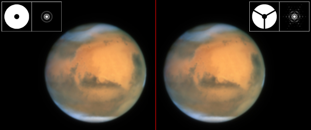
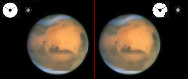
Figure 5b: An instrument with 20% central obstruction (left) compared with an instrument that additionally
has a three-vane spider of 1.5% mirror diameter. The influence on planetary contrast is negligible.

Even really massive supporting "vanes", that reach into the optical path, have very little influence on planetary conrast. The geometry of Figure 6a is often found in lightweight (robotic) telescopes, that carry an electronic camera instead of a secondary mirror. The camera (or the secondary optical component) is supported by a tripod that reaches directly from the cell of the main mirror to the first focus. The geometry of Fig. 7a would be for a tetrapod respectively.
Following the simulations, a rule of thumb for the vanes would be: a three-vane spider with vanes with diameter under 5% of the linear diameter of the mirror is uncritical for the contrast in planetary observations - that is a much higher value than normally
assumed! For a four-vane spider, this value should be lower than 3%.

Figure 6a: 20% central obstruction with vanes of 5% of the diameter of the main entrance pupil and the resulting diffraction pattern.

Figure 6b: The loss in contrast for such massive vanes is astonishingly low, even though the influence on the diffraction pattern (corresponding to the view of a star) is prominent.

Figure 7a: a four vane spider of 5% clearly has more influence on the diffraction pattern than a three vane spider of 5%.

Figure 7b: Four supporting structures of the same size as in Figure 6a will result in a somewhat lower conrast, due to the higher amount of diffracted light outside the airy disk.

When building optical instruments, we often have to decide if structures like mirror clamps or the focuser should be allowed to reach into the optical path, or if we should spend some effort to prevent this, sometimes at the cost of a higher weight of the instrument. In Figure 7a a theoretical instrument with many constructive structures reaching into the optical path is presented, together with the influence on the diffraction pattern.

Figure 8a: an instrument with spider and secondary (top), compared with a theoretical instrument with several additional structures reaching into the optical path, like a focuser, vane mountings, mirror clamps, a heating cable for the secondary and some screws (bottom).

Figure 8b: the loss in surface contrast for the instrument with all the structures reaching heavily into the optical path is quite low.

When discussing the influence of vanes on the image, we have neglected the diffraction figures far away from bright objects like stars up to now. In practice, they have no influence on planetary contrast, but they are visible because of the immense dynamic of the human eye. This dynamic is not used when observing planetary surfaces.
To give a realistic view of these diffraction figures that often show up in rainbow colors, I have simulated the wide field views in color.

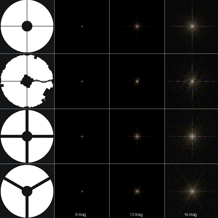
$diffraction pattern of different vanes$

Diffraction pattern of several vane configurations. The field of view is 60" (arcseconds) wide, again simulated for a 400mm diameter objective. At left the geometry of the obstruction is shown, the three images show simulated views with a dynamic range from black to white of 8 magnitudes, 12 magnitudes and 16 magnitudes, from left to right.
Upper row: a four vane spider of 0.4%, corresponding to the use of 1.6mm steel sheets for the vanes on a 400mm reflector.
Second row: again the 0.4% spider, but additionally with many other mechanical parts that reach into the optical path.
Third row: a four vane spider of 5%, corresponding to 20mm supporting tubes for instance.
Fourth row: a three vane spider of 5%. We get six diffraction spikes, but they are less bright than for four vanes.

Software used
For the simulation of the diffraction pattern I use a program I developed some time ago in Microsoft Visual C++. In fact, I got it working quite well, but due to lack in time and consquently a lack in programming experience it never reached a state of user friendlyness that I could publish it. I tested the software very critical and I am very shure that the simulations are correct.

Testing the program
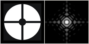
One critical test among others was the simulation of a complicated apodizer disk from literature, that was developed for a search for extraterrestrial planets close to stars on the proposed and meanwhile cancelled NASA space telescope "Terrestial Planet Finder -C". The complex apodizer diffracts most of the light, that normally falls into the diffraction rings, to other directions. This results in a diffraction pattern that has the diffraction rings suppressed by several magnitudes within a certain zone around the central maximum, enabling an excellent contrast for a search for faint objacts close to the star observed, on the expense of having strong diffraction structures in a zone around 90° to this orientation.
This apodizer, among other interesting ones, was developed and published by N. Jeremy Kasdin et al.:
N. J. Kasdin et al, “The Shaped Pupil Coronagraph For Planet Finding Coroangraphy: Optimization, Sensitivity and Laboratory Testing,” Proc. SPIE 5487, 1312-1321 (2004). Link (pdf).
I simulated the six pupil optimized mask from figure 6:

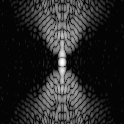
$diffraction pattern of a six pupil mask rom Kasdin et al$

Result from the simulation of the "six pupil optimized mask" from figure 6 left from the publication of N. J. Kasdin et al. It is very close to the result of their own simulation, that is shown in figure 6 right. The dynamic range from black to white is 14 mag.
Tests like this support my confidence in the program.