 |
|
|
|
Simulation of Sidescan Transducer
Arrays
|
| Page: 1, 2, 3 |
|
|
Figure
3a shows the sound projecting plane of an array of fishfinder
transducers how they are typically set up by amateur sidescan makers
to build a sidescan sonar. Since
each transducer with 44mm diameter is enclosed in a housing with
perhaps 60mm diameter the transducers are regularly spaced at this
distance as a minimum.
|
|
|

|
Figure 2a:
Transducer Array, 180mm long
|
|
|
|
Figure 2b:
calculated polar plot for the 180mm transducer array of Fig. 2a
working at 50kHz.
58% of the
emitted energy is concentrated in the central lobe that is 6.3°
wide.
|
|
|
|
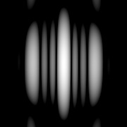
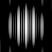
Figure
2c: two-dimensional energy distribution (soundfield) of the transducer
in Fig.2a Fieldsize:
120° x 120°, 25dB dynamic from white to black
|
|
|
|
As
to be expected
the soundpattern looks much more "sidescan sonar like", but
in comparison to the soundpattern of the real sidescan transducer of
Fig. 1a we discern some disadvantages of such a setup: The
central
lobe is much broader than the one in Fig. 1b and very strong sidelobes
arise. Strong sidelobes may lead to ghost-pattern and a loss of
contrast in the images and,
what is even more important, less amount of energy is concentrated in
the central lobe leading to a reduced range.
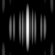
To obtain a narrower central lobe we could distribute the four
transducer in a longer array, but as can be seen in the
resulting Beampattern (Figures 3b and 3c) this leads to even more
energy
being lost in the sidelobes.
|
|

|
Figure 3a:
300mm long transducer array
|
|
|
|
Figure 3b:
polar plot for 300mm transducer array of Fig. 3a working at 50kHz.
Only 35% of the
emitted energy is concentrated in the 3.4° wide central lobe, 65%
is spread over the sidelobes.
|
|
|
|
Figure
3c: 2-D soundfield of the transducer in Fig.3a at 50kHz, Fieldsize:
120° x 120°, 25dB dynamic
|
|
|
|
Although
the
transducer is far from being perfect we
could build a fishfinder-array this way or the way in Fig. 2a and try
how
it performs, but as I will show we can do it much better with little
changes.
From the optical
analogon of the diffraction grating we know that we have to space the
diffracting structures very regularly to concentrate as much energy as
possible in the sidelobes (called first, second, ... order in optics);
only in these sidelobes the desired wavelength dispersion occurs.
Transferred to our transducer this means that, if we are forced to use
more or less widely spaced individual transducers in a row,
it is not a good idea to
space them regularly. An irregularly spaced array should help to
suppress the sidelobes. I ran some simulations to check this idea. |
|

|
Figure 3a:
Irregularly spaced transducer array, 300mm long
|
|
|
|
Figure 3b:
polar plot for 300mm irregularly spaced transducer array of Fig. 3a
working at
50kHz.
72% of the
emitted energy is concentrated in the 3.4° wide central lobe.
|
|
|
|
Figure
3c: 2-D soundfield of the irregularly spaced transducer in Fig.3a
Fieldsize:
120° x 120°, dynamik of 25 dB
|
|
|
|
The
array displayed in Fig.3a is, with the outer transducers spaced at
300mm,
as long as the one in Fig.2a, but the two inner transducers are
arranged
in a way that there are no regular distances. If we investigate the
simulated beampattern we find that the central lobe is as small as for
the regularly spaced 300mm array, but the sidelobes are much weaker.
The
energy concentrated in the central lobe with 72% is twice as high as
for the evenly spaced 300mm array that was 35%, and it is even
considerably higher than for the 180 mm array that gave 58%! By simply
spacing the
transducers irregularly we only have advantages, a narrower and
stronger central lobe and weaker sidelobes. This undoubtedly will
lead to a transducer that gives a better horizontal resolution,
stronger signals, higher range and better contrast.
We will certainly never reach the contrast and range of a good sidescan
transducer, since a considerable larger amount of energy is lost in the
sidelobes of our array and we will always have a diffuse background
from the sidelobes that lowers the contrast, but this is the price we
have to pay for the advantage of a cheap system compared to a
semi-professional or professiomal sidescan sonar system.
The 300mm array shown in Fig.3a is already optimized concerning the
positions of the transducers. I ran a lot of simulations on the try
and error principle to find this geometry to be the best. With the left
transducer being the number one and the right the number four we have
1->4 = 300mm, 1->3 = 150mm, and 1->2 = 65mm, the numbers given
are
always measured center to center.This kind of Transducer Array is
called a "Thinned Array".
Running the array at
200kHz
There is more good news concerning the arrays: if it is optimized
for 50kHz it is also optimized for other frequencies like 200kHz.
Figure 3d shows the beampattern and soundfield of the transducer
from Fig. 3a running at 200kHz. What is also clearly visible is the
narrow vertical width of the central lobe leading to a need of an exact
adjustment of the downtild angle; but even then the narrow vertical
beam
may lead to
restrictions in the imaged portion of the seafloor.
|
|
|
Figure 3d:
300mm transducer array of Fig. 3a working at 200kHz.
72% of the
emitted energy is concentrated in the 0.9° wide central lobe. The
inset shows the 2D soundfield at a fieldsize of 120°x120° and
25dB dynamic
|
|
|
Making it longer?
The wish for a narrow central lobe may lead to the idea to make the
array even longer, but this always leads to less energy concentrated in
the central lobe. An optimized transducer with 400mm length turned out
to be one with the values 1->4 = 400mm, 1->3 =
205mm, and 1->2 = 95mm; the central lobe holds 55% and is 2.7°
wide
at the -3dB point. An optimized transducer of 500mm length gives a
central lobe that, with 2.3° is nearly as narrow as the one of the
perfect
sidescan mentioned at the beginning, but it holds only 42% of the
energy. The distance values are: 500mm, 290mm and 100mm. A way out of
this
dilemma could only be to use more transducer, for instance six as a
first try.
Practical Tests
I am planning to build a system on this principle, I already have
many components, but time is always a problem, as most of us will know.
If I have any results I will publish them here.
|
|
Next
Page:
Simulation af a damaged
and
a "bad" Sidescan Sonar Transducer
|